WeatherBench 2 Evaluation Quickstart
In this notebook, we will cover the basic functionality of the WeatherBench evaluation framework.
The WeatherBench evaluation framework takes two datasets for forecast and ground truth (called obs, even though reanalysis datasets like ERA5 are not observations), computes and saves the specified metrics.
Here, we will evalute ECMWF’s HRES forecast against ERA5.
# Pip might complain about the Pandas version. The notebook should still work as expected.
!pip install git+https://github.com/google-research/weatherbench2.git
import apache_beam   # Needs to be imported separately to avoid TypingError
import weatherbench2
import xarray as xr
# Run the code below to access cloud data on Colab!
# from google.colab import auth
# auth.authenticate_user()
Specify input datasets
Let’s take a look at the datasets. Currently, the WeatherBench pipeline requires all input dataset to be stored as Zarr files.
forecast_path = 'gs://weatherbench2/datasets/hres/2016-2022-0012-64x32_equiangular_conservative.zarr'
obs_path = 'gs://weatherbench2/datasets/era5/1959-2022-6h-64x32_equiangular_conservative.zarr'
climatology_path = 'gs://weatherbench2/datasets/era5-hourly-climatology/1990-2019_6h_64x32_equiangular_conservative.zarr'
Generally, we follow ECMWF’s naming conventions for the input files.
time[np.datetime64]: Time at forecast is initializedlead_timeorprediction_timedelta[np.timedelta64]: Lead timelatitude[float]: Latitudes from -90 to 90longitude[float]: Longitudes from 0 to 360level[hPa]: Pressure levels (optional)
We don’t actually need to open the forecast and obs datasets at this point, but we will do so here to see their structure.
xr.open_zarr(forecast_path)
<xarray.Dataset>
Dimensions:                   (time: 5114, prediction_timedelta: 41,
                               longitude: 64, latitude: 32, level: 13)
Coordinates:
  * latitude                  (latitude) float64 -87.19 -81.56 ... 81.56 87.19
  * level                     (level) int32 50 100 150 200 ... 700 850 925 1000
  * longitude                 (longitude) float64 0.0 5.625 ... 348.8 354.4
  * prediction_timedelta      (prediction_timedelta) timedelta64[ns] 00:00:00...
  * time                      (time) datetime64[ns] 2016-01-01 ... 2022-12-31...
Data variables: (12/16)
    10m_u_component_of_wind   (time, prediction_timedelta, longitude, latitude) float32 dask.array<chunksize=(4, 1, 64, 32), meta=np.ndarray>
    10m_v_component_of_wind   (time, prediction_timedelta, longitude, latitude) float32 dask.array<chunksize=(4, 1, 64, 32), meta=np.ndarray>
    10m_wind_speed            (time, prediction_timedelta, longitude, latitude) float32 dask.array<chunksize=(4, 1, 64, 32), meta=np.ndarray>
    2m_temperature            (time, prediction_timedelta, longitude, latitude) float32 dask.array<chunksize=(4, 1, 64, 32), meta=np.ndarray>
    geopotential              (time, prediction_timedelta, level, longitude, latitude) float32 dask.array<chunksize=(4, 1, 13, 64, 32), meta=np.ndarray>
    mean_sea_level_pressure   (time, prediction_timedelta, longitude, latitude) float32 dask.array<chunksize=(4, 1, 64, 32), meta=np.ndarray>
    ...                        ...
    total_precipitation_24hr  (time, prediction_timedelta, longitude, latitude) float32 dask.array<chunksize=(4, 1, 64, 32), meta=np.ndarray>
    total_precipitation_6hr   (time, prediction_timedelta, longitude, latitude) float32 dask.array<chunksize=(4, 1, 64, 32), meta=np.ndarray>
    u_component_of_wind       (time, prediction_timedelta, level, longitude, latitude) float32 dask.array<chunksize=(4, 1, 13, 64, 32), meta=np.ndarray>
    v_component_of_wind       (time, prediction_timedelta, level, longitude, latitude) float32 dask.array<chunksize=(4, 1, 13, 64, 32), meta=np.ndarray>
    vertical_velocity         (time, prediction_timedelta, level, longitude, latitude) float32 dask.array<chunksize=(4, 1, 13, 64, 32), meta=np.ndarray>
wind_speed (time, prediction_timedelta, level, longitude, latitude) float32 dask.array<chunksize=(4, 1, 13, 64, 32), meta=np.ndarray>- time: 5114
- prediction_timedelta: 41
- longitude: 64
- latitude: 32
- level: 13
- latitude(latitude)float64-87.19 -81.56 ... 81.56 87.19
array([-87.1875, -81.5625, -75.9375, -70.3125, -64.6875, -59.0625, -53.4375, -47.8125, -42.1875, -36.5625, -30.9375, -25.3125, -19.6875, -14.0625, -8.4375, -2.8125, 2.8125, 8.4375, 14.0625, 19.6875, 25.3125, 30.9375, 36.5625, 42.1875, 47.8125, 53.4375, 59.0625, 64.6875, 70.3125, 75.9375, 81.5625, 87.1875]) - level(level)int3250 100 150 200 ... 700 850 925 1000
array([ 50, 100, 150, 200, 250, 300, 400, 500, 600, 700, 850, 925, 1000], dtype=int32) - longitude(longitude)float640.0 5.625 11.25 ... 348.8 354.4
array([ 0. , 5.625, 11.25 , 16.875, 22.5 , 28.125, 33.75 , 39.375, 45. , 50.625, 56.25 , 61.875, 67.5 , 73.125, 78.75 , 84.375, 90. , 95.625, 101.25 , 106.875, 112.5 , 118.125, 123.75 , 129.375, 135. , 140.625, 146.25 , 151.875, 157.5 , 163.125, 168.75 , 174.375, 180. , 185.625, 191.25 , 196.875, 202.5 , 208.125, 213.75 , 219.375, 225. , 230.625, 236.25 , 241.875, 247.5 , 253.125, 258.75 , 264.375, 270. , 275.625, 281.25 , 286.875, 292.5 , 298.125, 303.75 , 309.375, 315. , 320.625, 326.25 , 331.875, 337.5 , 343.125, 348.75 , 354.375]) - prediction_timedelta(prediction_timedelta)timedelta64[ns]0 days 00:00:00 ... 10 days 00:0...
- long_name :
- time since forecast_reference_time
- standard_name :
- forecast_period
array([ 0, 21600000000000, 43200000000000, 64800000000000, 86400000000000, 108000000000000, 129600000000000, 151200000000000, 172800000000000, 194400000000000, 216000000000000, 237600000000000, 259200000000000, 280800000000000, 302400000000000, 324000000000000, 345600000000000, 367200000000000, 388800000000000, 410400000000000, 432000000000000, 453600000000000, 475200000000000, 496800000000000, 518400000000000, 540000000000000, 561600000000000, 583200000000000, 604800000000000, 626400000000000, 648000000000000, 669600000000000, 691200000000000, 712800000000000, 734400000000000, 756000000000000, 777600000000000, 799200000000000, 820800000000000, 842400000000000, 864000000000000], dtype='timedelta64[ns]') - time(time)datetime64[ns]2016-01-01 ... 2022-12-31T12:00:00
- long_name :
- initial time of forecast
- standard_name :
- forecast_reference_time
array(['2016-01-01T00:00:00.000000000', '2016-01-01T12:00:00.000000000',
       '2016-01-02T00:00:00.000000000', ..., '2022-12-30T12:00:00.000000000',
       '2022-12-31T00:00:00.000000000', '2022-12-31T12:00:00.000000000'],
      dtype='datetime64[ns]')
- 10m_u_component_of_wind(time, prediction_timedelta, longitude, latitude)float32dask.array<chunksize=(4, 1, 64, 32), meta=np.ndarray>
- long_name :
- 10 metre U wind component
- short_name :
- u10
- standard_name :
- unknown
- units :
- m s**-1
Array Chunk Bytes 1.60 GiB 32.00 kiB Shape (5114, 41, 64, 32) (4, 1, 64, 32) Dask graph 52439 chunks in 2 graph layers Data type float32 numpy.ndarray - 10m_v_component_of_wind(time, prediction_timedelta, longitude, latitude)float32dask.array<chunksize=(4, 1, 64, 32), meta=np.ndarray>
- long_name :
- 10 metre V wind component
- short_name :
- v10
- standard_name :
- unknown
- units :
- m s**-1
Array Chunk Bytes 1.60 GiB 32.00 kiB Shape (5114, 41, 64, 32) (4, 1, 64, 32) Dask graph 52439 chunks in 2 graph layers Data type float32 numpy.ndarray - 10m_wind_speed(time, prediction_timedelta, longitude, latitude)float32dask.array<chunksize=(4, 1, 64, 32), meta=np.ndarray>
Array Chunk Bytes 1.60 GiB 32.00 kiB Shape (5114, 41, 64, 32) (4, 1, 64, 32) Dask graph 52439 chunks in 2 graph layers Data type float32 numpy.ndarray - 2m_temperature(time, prediction_timedelta, longitude, latitude)float32dask.array<chunksize=(4, 1, 64, 32), meta=np.ndarray>
- long_name :
- 2 metre temperature
- short_name :
- t2m
- standard_name :
- unknown
- units :
- K
Array Chunk Bytes 1.60 GiB 32.00 kiB Shape (5114, 41, 64, 32) (4, 1, 64, 32) Dask graph 52439 chunks in 2 graph layers Data type float32 numpy.ndarray - geopotential(time, prediction_timedelta, level, longitude, latitude)float32dask.array<chunksize=(4, 1, 13, 64, 32), meta=np.ndarray>
- long_name :
- Geopotential
- short_name :
- z
- standard_name :
- geopotential
- units :
- m**2 s**-2
Array Chunk Bytes 20.80 GiB 416.00 kiB Shape (5114, 41, 13, 64, 32) (4, 1, 13, 64, 32) Dask graph 52439 chunks in 2 graph layers Data type float32 numpy.ndarray - mean_sea_level_pressure(time, prediction_timedelta, longitude, latitude)float32dask.array<chunksize=(4, 1, 64, 32), meta=np.ndarray>
- long_name :
- Mean sea level pressure
- short_name :
- msl
- standard_name :
- air_pressure_at_mean_sea_level
- units :
- Pa
Array Chunk Bytes 1.60 GiB 32.00 kiB Shape (5114, 41, 64, 32) (4, 1, 64, 32) Dask graph 52439 chunks in 2 graph layers Data type float32 numpy.ndarray - specific_humidity(time, prediction_timedelta, level, longitude, latitude)float32dask.array<chunksize=(4, 1, 13, 64, 32), meta=np.ndarray>
- long_name :
- Specific humidity
- short_name :
- q
- standard_name :
- specific_humidity
- units :
- kg kg**-1
Array Chunk Bytes 20.80 GiB 416.00 kiB Shape (5114, 41, 13, 64, 32) (4, 1, 13, 64, 32) Dask graph 52439 chunks in 2 graph layers Data type float32 numpy.ndarray - surface_pressure(time, prediction_timedelta, longitude, latitude)float32dask.array<chunksize=(4, 1, 64, 32), meta=np.ndarray>
- long_name :
- Surface pressure
- short_name :
- sp
- standard_name :
- surface_air_pressure
- units :
- Pa
Array Chunk Bytes 1.60 GiB 32.00 kiB Shape (5114, 41, 64, 32) (4, 1, 64, 32) Dask graph 52439 chunks in 2 graph layers Data type float32 numpy.ndarray - temperature(time, prediction_timedelta, level, longitude, latitude)float32dask.array<chunksize=(4, 1, 13, 64, 32), meta=np.ndarray>
- long_name :
- Temperature
- short_name :
- t
- standard_name :
- air_temperature
- units :
- K
Array Chunk Bytes 20.80 GiB 416.00 kiB Shape (5114, 41, 13, 64, 32) (4, 1, 13, 64, 32) Dask graph 52439 chunks in 2 graph layers Data type float32 numpy.ndarray - total_precipitation(time, prediction_timedelta, longitude, latitude)float32dask.array<chunksize=(4, 1, 64, 32), meta=np.ndarray>
- long_name :
- Total precipitation
- short_name :
- tp
- standard_name :
- unknown
- units :
- m
Array Chunk Bytes 1.60 GiB 32.00 kiB Shape (5114, 41, 64, 32) (4, 1, 64, 32) Dask graph 52439 chunks in 2 graph layers Data type float32 numpy.ndarray - total_precipitation_24hr(time, prediction_timedelta, longitude, latitude)float32dask.array<chunksize=(4, 1, 64, 32), meta=np.ndarray>
Array Chunk Bytes 1.60 GiB 32.00 kiB Shape (5114, 41, 64, 32) (4, 1, 64, 32) Dask graph 52439 chunks in 2 graph layers Data type float32 numpy.ndarray - total_precipitation_6hr(time, prediction_timedelta, longitude, latitude)float32dask.array<chunksize=(4, 1, 64, 32), meta=np.ndarray>
Array Chunk Bytes 1.60 GiB 32.00 kiB Shape (5114, 41, 64, 32) (4, 1, 64, 32) Dask graph 52439 chunks in 2 graph layers Data type float32 numpy.ndarray - u_component_of_wind(time, prediction_timedelta, level, longitude, latitude)float32dask.array<chunksize=(4, 1, 13, 64, 32), meta=np.ndarray>
- long_name :
- U component of wind
- short_name :
- u
- standard_name :
- eastward_wind
- units :
- m s**-1
Array Chunk Bytes 20.80 GiB 416.00 kiB Shape (5114, 41, 13, 64, 32) (4, 1, 13, 64, 32) Dask graph 52439 chunks in 2 graph layers Data type float32 numpy.ndarray - v_component_of_wind(time, prediction_timedelta, level, longitude, latitude)float32dask.array<chunksize=(4, 1, 13, 64, 32), meta=np.ndarray>
- long_name :
- V component of wind
- short_name :
- v
- standard_name :
- northward_wind
- units :
- m s**-1
Array Chunk Bytes 20.80 GiB 416.00 kiB Shape (5114, 41, 13, 64, 32) (4, 1, 13, 64, 32) Dask graph 52439 chunks in 2 graph layers Data type float32 numpy.ndarray - vertical_velocity(time, prediction_timedelta, level, longitude, latitude)float32dask.array<chunksize=(4, 1, 13, 64, 32), meta=np.ndarray>
- long_name :
- Vertical velocity
- short_name :
- w
- standard_name :
- lagrangian_tendency_of_air_pressure
- units :
- Pa s**-1
Array Chunk Bytes 20.80 GiB 416.00 kiB Shape (5114, 41, 13, 64, 32) (4, 1, 13, 64, 32) Dask graph 52439 chunks in 2 graph layers Data type float32 numpy.ndarray - wind_speed(time, prediction_timedelta, level, longitude, latitude)float32dask.array<chunksize=(4, 1, 13, 64, 32), meta=np.ndarray>
Array Chunk Bytes 20.80 GiB 416.00 kiB Shape (5114, 41, 13, 64, 32) (4, 1, 13, 64, 32) Dask graph 52439 chunks in 2 graph layers Data type float32 numpy.ndarray
- latitudePandasIndex
PandasIndex(Index([ -87.18750000000003, -81.56250000000001, -75.9375, -70.31249999999999, -64.68750000000001, -59.0625, -53.4375, -47.8125, -42.1875, -36.5625, -30.937499999999996, -25.312500000000004, -19.687499999999996, -14.062499999999991, -8.437499999999996, -2.812500000000003, 2.812500000000003, 8.437500000000009, 14.062500000000004, 19.687499999999996, 25.312500000000004, 30.93750000000001, 36.562499999999986, 42.1875, 47.8125, 53.4375, 59.062500000000014, 64.68750000000001, 70.3125, 75.9375, 81.56249999999997, 87.18750000000003], dtype='float64', name='latitude')) - levelPandasIndex
PandasIndex(Index([50, 100, 150, 200, 250, 300, 400, 500, 600, 700, 850, 925, 1000], dtype='int32', name='level'))
- longitudePandasIndex
PandasIndex(Index([ 0.0, 5.625, 11.25, 16.875, 22.5, 28.125, 33.75, 39.375, 45.0, 50.625, 56.25, 61.87499999999999, 67.5, 73.125, 78.75, 84.375, 90.0, 95.625, 101.25, 106.875, 112.5, 118.125, 123.74999999999999, 129.375, 135.0, 140.625, 146.25, 151.875, 157.5, 163.125, 168.75, 174.375, 180.0, 185.625, 191.25, 196.875, 202.5, 208.125, 213.75, 219.375, 225.0, 230.62499999999997, 236.25, 241.875, 247.49999999999997, 253.125, 258.75, 264.375, 270.0, 275.625, 281.25, 286.875, 292.5, 298.125, 303.75, 309.375, 315.0, 320.625, 326.25, 331.875, 337.5, 343.125, 348.75, 354.375], dtype='float64', name='longitude')) - prediction_timedeltaPandasIndex
PandasIndex(TimedeltaIndex([ '0 days 00:00:00', '0 days 06:00:00', '0 days 12:00:00', '0 days 18:00:00', '1 days 00:00:00', '1 days 06:00:00', '1 days 12:00:00', '1 days 18:00:00', '2 days 00:00:00', '2 days 06:00:00', '2 days 12:00:00', '2 days 18:00:00', '3 days 00:00:00', '3 days 06:00:00', '3 days 12:00:00', '3 days 18:00:00', '4 days 00:00:00', '4 days 06:00:00', '4 days 12:00:00', '4 days 18:00:00', '5 days 00:00:00', '5 days 06:00:00', '5 days 12:00:00', '5 days 18:00:00', '6 days 00:00:00', '6 days 06:00:00', '6 days 12:00:00', '6 days 18:00:00', '7 days 00:00:00', '7 days 06:00:00', '7 days 12:00:00', '7 days 18:00:00', '8 days 00:00:00', '8 days 06:00:00', '8 days 12:00:00', '8 days 18:00:00', '9 days 00:00:00', '9 days 06:00:00', '9 days 12:00:00', '9 days 18:00:00', '10 days 00:00:00'], dtype='timedelta64[ns]', name='prediction_timedelta', freq=None)) - timePandasIndex
PandasIndex(DatetimeIndex(['2016-01-01 00:00:00', '2016-01-01 12:00:00',
               '2016-01-02 00:00:00', '2016-01-02 12:00:00',
               '2016-01-03 00:00:00', '2016-01-03 12:00:00',
               '2016-01-04 00:00:00', '2016-01-04 12:00:00',
               '2016-01-05 00:00:00', '2016-01-05 12:00:00',
               ...
               '2022-12-27 00:00:00', '2022-12-27 12:00:00',
               '2022-12-28 00:00:00', '2022-12-28 12:00:00',
               '2022-12-29 00:00:00', '2022-12-29 12:00:00',
               '2022-12-30 00:00:00', '2022-12-30 12:00:00',
               '2022-12-31 00:00:00', '2022-12-31 12:00:00'],
              dtype='datetime64[ns]', name='time', length=5114, freq=None))
xr.open_zarr(obs_path)
<xarray.Dataset>
Dimensions:                                           (time: 92044,
                                                       longitude: 64,
                                                       latitude: 32, level: 13)
Coordinates:
  * latitude                                          (latitude) float64 -87....
  * level                                             (level) int64 50 ... 1000
  * longitude                                         (longitude) float64 0.0...
  * time                                              (time) datetime64[ns] 1...
Data variables: (12/38)
    10m_u_component_of_wind                           (time, longitude, latitude) float32 dask.array<chunksize=(100, 64, 32), meta=np.ndarray>
    10m_v_component_of_wind                           (time, longitude, latitude) float32 dask.array<chunksize=(100, 64, 32), meta=np.ndarray>
    10m_wind_speed                                    (time, longitude, latitude) float32 dask.array<chunksize=(100, 64, 32), meta=np.ndarray>
    2m_temperature                                    (time, longitude, latitude) float32 dask.array<chunksize=(100, 64, 32), meta=np.ndarray>
    angle_of_sub_gridscale_orography                  (longitude, latitude) float32 dask.array<chunksize=(64, 32), meta=np.ndarray>
    anisotropy_of_sub_gridscale_orography             (longitude, latitude) float32 dask.array<chunksize=(64, 32), meta=np.ndarray>
    ...                                                ...
    type_of_high_vegetation                           (longitude, latitude) float32 dask.array<chunksize=(64, 32), meta=np.ndarray>
    type_of_low_vegetation                            (longitude, latitude) float32 dask.array<chunksize=(64, 32), meta=np.ndarray>
    u_component_of_wind                               (time, level, longitude, latitude) float32 dask.array<chunksize=(100, 13, 64, 32), meta=np.ndarray>
    v_component_of_wind                               (time, level, longitude, latitude) float32 dask.array<chunksize=(100, 13, 64, 32), meta=np.ndarray>
    vertical_velocity                                 (time, level, longitude, latitude) float32 dask.array<chunksize=(100, 13, 64, 32), meta=np.ndarray>
wind_speed (time, level, longitude, latitude) float32 dask.array<chunksize=(100, 13, 64, 32), meta=np.ndarray>- time: 92044
- longitude: 64
- latitude: 32
- level: 13
- latitude(latitude)float64-87.19 -81.56 ... 81.56 87.19
array([-87.1875, -81.5625, -75.9375, -70.3125, -64.6875, -59.0625, -53.4375, -47.8125, -42.1875, -36.5625, -30.9375, -25.3125, -19.6875, -14.0625, -8.4375, -2.8125, 2.8125, 8.4375, 14.0625, 19.6875, 25.3125, 30.9375, 36.5625, 42.1875, 47.8125, 53.4375, 59.0625, 64.6875, 70.3125, 75.9375, 81.5625, 87.1875]) - level(level)int6450 100 150 200 ... 700 850 925 1000
array([ 50, 100, 150, 200, 250, 300, 400, 500, 600, 700, 850, 925, 1000]) - longitude(longitude)float640.0 5.625 11.25 ... 348.8 354.4
array([ 0. , 5.625, 11.25 , 16.875, 22.5 , 28.125, 33.75 , 39.375, 45. , 50.625, 56.25 , 61.875, 67.5 , 73.125, 78.75 , 84.375, 90. , 95.625, 101.25 , 106.875, 112.5 , 118.125, 123.75 , 129.375, 135. , 140.625, 146.25 , 151.875, 157.5 , 163.125, 168.75 , 174.375, 180. , 185.625, 191.25 , 196.875, 202.5 , 208.125, 213.75 , 219.375, 225. , 230.625, 236.25 , 241.875, 247.5 , 253.125, 258.75 , 264.375, 270. , 275.625, 281.25 , 286.875, 292.5 , 298.125, 303.75 , 309.375, 315. , 320.625, 326.25 , 331.875, 337.5 , 343.125, 348.75 , 354.375]) - time(time)datetime64[ns]1959-01-01 ... 2021-12-31T18:00:00
array(['1959-01-01T00:00:00.000000000', '1959-01-01T06:00:00.000000000',
       '1959-01-01T12:00:00.000000000', ..., '2021-12-31T06:00:00.000000000',
       '2021-12-31T12:00:00.000000000', '2021-12-31T18:00:00.000000000'],
      dtype='datetime64[ns]')
- 10m_u_component_of_wind(time, longitude, latitude)float32dask.array<chunksize=(100, 64, 32), meta=np.ndarray>
- long_name :
- 10 metre U wind component
- short_name :
- u10
- units :
- m s**-1
Array Chunk Bytes 719.09 MiB 800.00 kiB Shape (92044, 64, 32) (100, 64, 32) Dask graph 921 chunks in 2 graph layers Data type float32 numpy.ndarray - 10m_v_component_of_wind(time, longitude, latitude)float32dask.array<chunksize=(100, 64, 32), meta=np.ndarray>
- long_name :
- 10 metre V wind component
- short_name :
- v10
- units :
- m s**-1
Array Chunk Bytes 719.09 MiB 800.00 kiB Shape (92044, 64, 32) (100, 64, 32) Dask graph 921 chunks in 2 graph layers Data type float32 numpy.ndarray - 10m_wind_speed(time, longitude, latitude)float32dask.array<chunksize=(100, 64, 32), meta=np.ndarray>
Array Chunk Bytes 719.09 MiB 800.00 kiB Shape (92044, 64, 32) (100, 64, 32) Dask graph 921 chunks in 2 graph layers Data type float32 numpy.ndarray - 2m_temperature(time, longitude, latitude)float32dask.array<chunksize=(100, 64, 32), meta=np.ndarray>
- long_name :
- 2 metre temperature
- short_name :
- t2m
- units :
- K
Array Chunk Bytes 719.09 MiB 800.00 kiB Shape (92044, 64, 32) (100, 64, 32) Dask graph 921 chunks in 2 graph layers Data type float32 numpy.ndarray - angle_of_sub_gridscale_orography(longitude, latitude)float32dask.array<chunksize=(64, 32), meta=np.ndarray>
- long_name :
- Angle of sub-gridscale orography
- short_name :
- anor
- units :
- radians
Array Chunk Bytes 8.00 kiB 8.00 kiB Shape (64, 32) (64, 32) Dask graph 1 chunks in 2 graph layers Data type float32 numpy.ndarray - anisotropy_of_sub_gridscale_orography(longitude, latitude)float32dask.array<chunksize=(64, 32), meta=np.ndarray>
- long_name :
- Anisotropy of sub-gridscale orography
- short_name :
- isor
- units :
- ~
Array Chunk Bytes 8.00 kiB 8.00 kiB Shape (64, 32) (64, 32) Dask graph 1 chunks in 2 graph layers Data type float32 numpy.ndarray - geopotential(time, level, longitude, latitude)float32dask.array<chunksize=(100, 13, 64, 32), meta=np.ndarray>
- long_name :
- Geopotential
- short_name :
- z
- standard_name :
- geopotential
- units :
- m**2 s**-2
Array Chunk Bytes 9.13 GiB 10.16 MiB Shape (92044, 13, 64, 32) (100, 13, 64, 32) Dask graph 921 chunks in 2 graph layers Data type float32 numpy.ndarray - geopotential_at_surface(longitude, latitude)float32dask.array<chunksize=(64, 32), meta=np.ndarray>
- long_name :
- Geopotential
- short_name :
- z
- standard_name :
- geopotential
- units :
- m**2 s**-2
Array Chunk Bytes 8.00 kiB 8.00 kiB Shape (64, 32) (64, 32) Dask graph 1 chunks in 2 graph layers Data type float32 numpy.ndarray - high_vegetation_cover(longitude, latitude)float32dask.array<chunksize=(64, 32), meta=np.ndarray>
- long_name :
- High vegetation cover
- short_name :
- cvh
- units :
- (0 - 1)
Array Chunk Bytes 8.00 kiB 8.00 kiB Shape (64, 32) (64, 32) Dask graph 1 chunks in 2 graph layers Data type float32 numpy.ndarray - lake_cover(longitude, latitude)float32dask.array<chunksize=(64, 32), meta=np.ndarray>
- long_name :
- Lake cover
- short_name :
- cl
- units :
- (0 - 1)
Array Chunk Bytes 8.00 kiB 8.00 kiB Shape (64, 32) (64, 32) Dask graph 1 chunks in 2 graph layers Data type float32 numpy.ndarray - lake_depth(longitude, latitude)float32dask.array<chunksize=(64, 32), meta=np.ndarray>
- long_name :
- Lake total depth
- short_name :
- dl
- units :
- m
Array Chunk Bytes 8.00 kiB 8.00 kiB Shape (64, 32) (64, 32) Dask graph 1 chunks in 2 graph layers Data type float32 numpy.ndarray - land_sea_mask(longitude, latitude)float32dask.array<chunksize=(64, 32), meta=np.ndarray>
- long_name :
- Land-sea mask
- short_name :
- lsm
- standard_name :
- land_binary_mask
- units :
- (0 - 1)
Array Chunk Bytes 8.00 kiB 8.00 kiB Shape (64, 32) (64, 32) Dask graph 1 chunks in 2 graph layers Data type float32 numpy.ndarray - low_vegetation_cover(longitude, latitude)float32dask.array<chunksize=(64, 32), meta=np.ndarray>
- long_name :
- Low vegetation cover
- short_name :
- cvl
- units :
- (0 - 1)
Array Chunk Bytes 8.00 kiB 8.00 kiB Shape (64, 32) (64, 32) Dask graph 1 chunks in 2 graph layers Data type float32 numpy.ndarray - mean_sea_level_pressure(time, longitude, latitude)float32dask.array<chunksize=(100, 64, 32), meta=np.ndarray>
- long_name :
- Mean sea level pressure
- short_name :
- msl
- standard_name :
- air_pressure_at_mean_sea_level
- units :
- Pa
Array Chunk Bytes 719.09 MiB 800.00 kiB Shape (92044, 64, 32) (100, 64, 32) Dask graph 921 chunks in 2 graph layers Data type float32 numpy.ndarray - sea_ice_cover(time, longitude, latitude)float32dask.array<chunksize=(100, 64, 32), meta=np.ndarray>
- long_name :
- Sea ice area fraction
- short_name :
- siconc
- standard_name :
- sea_ice_area_fraction
- units :
- (0 - 1)
Array Chunk Bytes 719.09 MiB 800.00 kiB Shape (92044, 64, 32) (100, 64, 32) Dask graph 921 chunks in 2 graph layers Data type float32 numpy.ndarray - sea_surface_temperature(time, longitude, latitude)float32dask.array<chunksize=(100, 64, 32), meta=np.ndarray>
- long_name :
- Sea surface temperature
- short_name :
- sst
- units :
- K
Array Chunk Bytes 719.09 MiB 800.00 kiB Shape (92044, 64, 32) (100, 64, 32) Dask graph 921 chunks in 2 graph layers Data type float32 numpy.ndarray - slope_of_sub_gridscale_orography(longitude, latitude)float32dask.array<chunksize=(64, 32), meta=np.ndarray>
- long_name :
- Slope of sub-gridscale orography
- short_name :
- slor
- units :
- ~
Array Chunk Bytes 8.00 kiB 8.00 kiB Shape (64, 32) (64, 32) Dask graph 1 chunks in 2 graph layers Data type float32 numpy.ndarray - soil_type(longitude, latitude)float32dask.array<chunksize=(64, 32), meta=np.ndarray>
- long_name :
- Soil type
- short_name :
- slt
- units :
- ~
Array Chunk Bytes 8.00 kiB 8.00 kiB Shape (64, 32) (64, 32) Dask graph 1 chunks in 2 graph layers Data type float32 numpy.ndarray - specific_humidity(time, level, longitude, latitude)float32dask.array<chunksize=(100, 13, 64, 32), meta=np.ndarray>
- long_name :
- Specific humidity
- short_name :
- q
- standard_name :
- specific_humidity
- units :
- kg kg**-1
Array Chunk Bytes 9.13 GiB 10.16 MiB Shape (92044, 13, 64, 32) (100, 13, 64, 32) Dask graph 921 chunks in 2 graph layers Data type float32 numpy.ndarray - standard_deviation_of_filtered_subgrid_orography(longitude, latitude)float32dask.array<chunksize=(64, 32), meta=np.ndarray>
- long_name :
- Standard deviation of filtered subgrid orography
- short_name :
- sdfor
- units :
- m
Array Chunk Bytes 8.00 kiB 8.00 kiB Shape (64, 32) (64, 32) Dask graph 1 chunks in 2 graph layers Data type float32 numpy.ndarray - standard_deviation_of_orography(longitude, latitude)float32dask.array<chunksize=(64, 32), meta=np.ndarray>
- long_name :
- Standard deviation of orography
- short_name :
- sdor
- units :
- m
Array Chunk Bytes 8.00 kiB 8.00 kiB Shape (64, 32) (64, 32) Dask graph 1 chunks in 2 graph layers Data type float32 numpy.ndarray - surface_pressure(time, longitude, latitude)float32dask.array<chunksize=(100, 64, 32), meta=np.ndarray>
- long_name :
- Surface pressure
- short_name :
- sp
- standard_name :
- surface_air_pressure
- units :
- Pa
Array Chunk Bytes 719.09 MiB 800.00 kiB Shape (92044, 64, 32) (100, 64, 32) Dask graph 921 chunks in 2 graph layers Data type float32 numpy.ndarray - temperature(time, level, longitude, latitude)float32dask.array<chunksize=(100, 13, 64, 32), meta=np.ndarray>
- long_name :
- Temperature
- short_name :
- t
- standard_name :
- air_temperature
- units :
- K
Array Chunk Bytes 9.13 GiB 10.16 MiB Shape (92044, 13, 64, 32) (100, 13, 64, 32) Dask graph 921 chunks in 2 graph layers Data type float32 numpy.ndarray - toa_incident_solar_radiation(time, longitude, latitude)float32dask.array<chunksize=(100, 64, 32), meta=np.ndarray>
- long_name :
- TOA incident solar radiation
- short_name :
- tisr
- units :
- J m**-2
Array Chunk Bytes 719.09 MiB 800.00 kiB Shape (92044, 64, 32) (100, 64, 32) Dask graph 921 chunks in 2 graph layers Data type float32 numpy.ndarray - toa_incident_solar_radiation_12hr(time, longitude, latitude)float32dask.array<chunksize=(100, 64, 32), meta=np.ndarray>
- long_name :
- TOA incident solar radiation
- short_name :
- tisr
- units :
- J m**-2
Array Chunk Bytes 719.09 MiB 800.00 kiB Shape (92044, 64, 32) (100, 64, 32) Dask graph 921 chunks in 2 graph layers Data type float32 numpy.ndarray - toa_incident_solar_radiation_24hr(time, longitude, latitude)float32dask.array<chunksize=(100, 64, 32), meta=np.ndarray>
- long_name :
- TOA incident solar radiation
- short_name :
- tisr
- units :
- J m**-2
Array Chunk Bytes 719.09 MiB 800.00 kiB Shape (92044, 64, 32) (100, 64, 32) Dask graph 921 chunks in 2 graph layers Data type float32 numpy.ndarray - toa_incident_solar_radiation_6hr(time, longitude, latitude)float32dask.array<chunksize=(100, 64, 32), meta=np.ndarray>
- long_name :
- TOA incident solar radiation
- short_name :
- tisr
- units :
- J m**-2
Array Chunk Bytes 719.09 MiB 800.00 kiB Shape (92044, 64, 32) (100, 64, 32) Dask graph 921 chunks in 2 graph layers Data type float32 numpy.ndarray - total_cloud_cover(time, longitude, latitude)float32dask.array<chunksize=(100, 64, 32), meta=np.ndarray>
- long_name :
- Total cloud cover
- short_name :
- tcc
- standard_name :
- cloud_area_fraction
- units :
- (0 - 1)
Array Chunk Bytes 719.09 MiB 800.00 kiB Shape (92044, 64, 32) (100, 64, 32) Dask graph 921 chunks in 2 graph layers Data type float32 numpy.ndarray - total_column_water_vapour(time, longitude, latitude)float32dask.array<chunksize=(100, 64, 32), meta=np.ndarray>
- long_name :
- Total column vertically-integrated water vapour
- short_name :
- tcwv
- standard_name :
- lwe_thickness_of_atmosphere_mass_content_of_water_vapor
- units :
- kg m**-2
Array Chunk Bytes 719.09 MiB 800.00 kiB Shape (92044, 64, 32) (100, 64, 32) Dask graph 921 chunks in 2 graph layers Data type float32 numpy.ndarray - total_precipitation_12hr(time, longitude, latitude)float32dask.array<chunksize=(100, 64, 32), meta=np.ndarray>
- long_name :
- Total precipitation
- short_name :
- tp
- units :
- m
Array Chunk Bytes 719.09 MiB 800.00 kiB Shape (92044, 64, 32) (100, 64, 32) Dask graph 921 chunks in 2 graph layers Data type float32 numpy.ndarray - total_precipitation_24hr(time, longitude, latitude)float32dask.array<chunksize=(100, 64, 32), meta=np.ndarray>
- long_name :
- Total precipitation
- short_name :
- tp
- units :
- m
Array Chunk Bytes 719.09 MiB 800.00 kiB Shape (92044, 64, 32) (100, 64, 32) Dask graph 921 chunks in 2 graph layers Data type float32 numpy.ndarray - total_precipitation_6hr(time, longitude, latitude)float32dask.array<chunksize=(100, 64, 32), meta=np.ndarray>
- long_name :
- Total precipitation
- short_name :
- tp
- units :
- m
Array Chunk Bytes 719.09 MiB 800.00 kiB Shape (92044, 64, 32) (100, 64, 32) Dask graph 921 chunks in 2 graph layers Data type float32 numpy.ndarray - type_of_high_vegetation(longitude, latitude)float32dask.array<chunksize=(64, 32), meta=np.ndarray>
- long_name :
- Type of high vegetation
- short_name :
- tvh
- units :
- ~
Array Chunk Bytes 8.00 kiB 8.00 kiB Shape (64, 32) (64, 32) Dask graph 1 chunks in 2 graph layers Data type float32 numpy.ndarray - type_of_low_vegetation(longitude, latitude)float32dask.array<chunksize=(64, 32), meta=np.ndarray>
- long_name :
- Type of low vegetation
- short_name :
- tvl
- units :
- ~
Array Chunk Bytes 8.00 kiB 8.00 kiB Shape (64, 32) (64, 32) Dask graph 1 chunks in 2 graph layers Data type float32 numpy.ndarray - u_component_of_wind(time, level, longitude, latitude)float32dask.array<chunksize=(100, 13, 64, 32), meta=np.ndarray>
- long_name :
- U component of wind
- short_name :
- u
- standard_name :
- eastward_wind
- units :
- m s**-1
Array Chunk Bytes 9.13 GiB 10.16 MiB Shape (92044, 13, 64, 32) (100, 13, 64, 32) Dask graph 921 chunks in 2 graph layers Data type float32 numpy.ndarray - v_component_of_wind(time, level, longitude, latitude)float32dask.array<chunksize=(100, 13, 64, 32), meta=np.ndarray>
- long_name :
- V component of wind
- short_name :
- v
- standard_name :
- northward_wind
- units :
- m s**-1
Array Chunk Bytes 9.13 GiB 10.16 MiB Shape (92044, 13, 64, 32) (100, 13, 64, 32) Dask graph 921 chunks in 2 graph layers Data type float32 numpy.ndarray - vertical_velocity(time, level, longitude, latitude)float32dask.array<chunksize=(100, 13, 64, 32), meta=np.ndarray>
- long_name :
- Vertical velocity
- short_name :
- w
- standard_name :
- lagrangian_tendency_of_air_pressure
- units :
- Pa s**-1
Array Chunk Bytes 9.13 GiB 10.16 MiB Shape (92044, 13, 64, 32) (100, 13, 64, 32) Dask graph 921 chunks in 2 graph layers Data type float32 numpy.ndarray - wind_speed(time, level, longitude, latitude)float32dask.array<chunksize=(100, 13, 64, 32), meta=np.ndarray>
Array Chunk Bytes 9.13 GiB 10.16 MiB Shape (92044, 13, 64, 32) (100, 13, 64, 32) Dask graph 921 chunks in 2 graph layers Data type float32 numpy.ndarray
- latitudePandasIndex
PandasIndex(Index([ -87.18750000000003, -81.56250000000001, -75.9375, -70.31249999999999, -64.68750000000001, -59.0625, -53.4375, -47.8125, -42.1875, -36.5625, -30.937499999999996, -25.312500000000004, -19.687499999999996, -14.062499999999991, -8.437499999999996, -2.812500000000003, 2.812500000000003, 8.437500000000009, 14.062500000000004, 19.687499999999996, 25.312500000000004, 30.93750000000001, 36.562499999999986, 42.1875, 47.8125, 53.4375, 59.062500000000014, 64.68750000000001, 70.3125, 75.9375, 81.56249999999997, 87.18750000000003], dtype='float64', name='latitude')) - levelPandasIndex
PandasIndex(Index([50, 100, 150, 200, 250, 300, 400, 500, 600, 700, 850, 925, 1000], dtype='int64', name='level'))
- longitudePandasIndex
PandasIndex(Index([ 0.0, 5.625, 11.25, 16.875, 22.5, 28.125, 33.75, 39.375, 45.0, 50.625, 56.25, 61.87499999999999, 67.5, 73.125, 78.75, 84.375, 90.0, 95.625, 101.25, 106.875, 112.5, 118.125, 123.74999999999999, 129.375, 135.0, 140.625, 146.25, 151.875, 157.5, 163.125, 168.75, 174.375, 180.0, 185.625, 191.25, 196.875, 202.5, 208.125, 213.75, 219.375, 225.0, 230.62499999999997, 236.25, 241.875, 247.49999999999997, 253.125, 258.75, 264.375, 270.0, 275.625, 281.25, 286.875, 292.5, 298.125, 303.75, 309.375, 315.0, 320.625, 326.25, 331.875, 337.5, 343.125, 348.75, 354.375], dtype='float64', name='longitude')) - timePandasIndex
PandasIndex(DatetimeIndex(['1959-01-01 00:00:00', '1959-01-01 06:00:00',
               '1959-01-01 12:00:00', '1959-01-01 18:00:00',
               '1959-01-02 00:00:00', '1959-01-02 06:00:00',
               '1959-01-02 12:00:00', '1959-01-02 18:00:00',
               '1959-01-03 00:00:00', '1959-01-03 06:00:00',
               ...
               '2021-12-29 12:00:00', '2021-12-29 18:00:00',
               '2021-12-30 00:00:00', '2021-12-30 06:00:00',
               '2021-12-30 12:00:00', '2021-12-30 18:00:00',
               '2021-12-31 00:00:00', '2021-12-31 06:00:00',
               '2021-12-31 12:00:00', '2021-12-31 18:00:00'],
              dtype='datetime64[ns]', name='time', length=92044, freq=None))
Some metrics like the ACC also require a climatology file. Refer to the paper for details on how this is computed.
climatology = xr.open_zarr(climatology_path)
climatology
<xarray.Dataset>
Dimensions:                                      (hour: 4, dayofyear: 366,
                                                  longitude: 64, latitude: 32,
                                                  level: 13)
Coordinates:
  * dayofyear                                    (dayofyear) int64 1 2 ... 366
  * hour                                         (hour) int64 0 6 12 18
  * latitude                                     (latitude) float64 -87.19 .....
  * level                                        (level) int64 50 100 ... 1000
  * longitude                                    (longitude) float64 0.0 ... ...
Data variables: (12/28)
    10m_u_component_of_wind                      (hour, dayofyear, longitude, latitude) float32 dask.array<chunksize=(4, 366, 64, 32), meta=np.ndarray>
    10m_v_component_of_wind                      (hour, dayofyear, longitude, latitude) float32 dask.array<chunksize=(4, 366, 64, 32), meta=np.ndarray>
    10m_wind_speed                               (hour, dayofyear, longitude, latitude) float32 dask.array<chunksize=(4, 366, 64, 32), meta=np.ndarray>
    2m_temperature                               (hour, dayofyear, longitude, latitude) float32 dask.array<chunksize=(4, 366, 64, 32), meta=np.ndarray>
    geopotential                                 (hour, dayofyear, level, longitude, latitude) float32 dask.array<chunksize=(4, 366, 13, 64, 32), meta=np.ndarray>
    mean_sea_level_pressure                      (hour, dayofyear, longitude, latitude) float32 dask.array<chunksize=(4, 366, 64, 32), meta=np.ndarray>
    ...                                           ...
    total_precipitation_6hr_seeps_dry_fraction   (hour, dayofyear, longitude, latitude) float32 dask.array<chunksize=(4, 366, 64, 32), meta=np.ndarray>
    total_precipitation_6hr_seeps_threshold      (hour, dayofyear, longitude, latitude) float32 dask.array<chunksize=(4, 366, 64, 32), meta=np.ndarray>
    u_component_of_wind                          (hour, dayofyear, level, longitude, latitude) float32 dask.array<chunksize=(4, 366, 13, 64, 32), meta=np.ndarray>
    v_component_of_wind                          (hour, dayofyear, level, longitude, latitude) float32 dask.array<chunksize=(4, 366, 13, 64, 32), meta=np.ndarray>
    vertical_velocity                            (hour, dayofyear, level, longitude, latitude) float32 dask.array<chunksize=(4, 366, 13, 64, 32), meta=np.ndarray>
wind_speed (hour, dayofyear, level, longitude, latitude) float32 dask.array<chunksize=(4, 366, 13, 64, 32), meta=np.ndarray>- hour: 4
- dayofyear: 366
- longitude: 64
- latitude: 32
- level: 13
- dayofyear(dayofyear)int641 2 3 4 5 6 ... 362 363 364 365 366
array([ 1, 2, 3, ..., 364, 365, 366])
- hour(hour)int640 6 12 18
array([ 0, 6, 12, 18])
- latitude(latitude)float64-87.19 -81.56 ... 81.56 87.19
array([-87.1875, -81.5625, -75.9375, -70.3125, -64.6875, -59.0625, -53.4375, -47.8125, -42.1875, -36.5625, -30.9375, -25.3125, -19.6875, -14.0625, -8.4375, -2.8125, 2.8125, 8.4375, 14.0625, 19.6875, 25.3125, 30.9375, 36.5625, 42.1875, 47.8125, 53.4375, 59.0625, 64.6875, 70.3125, 75.9375, 81.5625, 87.1875]) - level(level)int6450 100 150 200 ... 700 850 925 1000
array([ 50, 100, 150, 200, 250, 300, 400, 500, 600, 700, 850, 925, 1000]) - longitude(longitude)float640.0 5.625 11.25 ... 348.8 354.4
array([  0.   ,   5.625,  11.25 ,  16.875,  22.5  ,  28.125,  33.75 ,  39.375,
        45.   ,  50.625,  56.25 ,  61.875,  67.5  ,  73.125,  78.75 ,  84.375,
        90.   ,  95.625, 101.25 , 106.875, 112.5  , 118.125, 123.75 , 129.375,
       135.   , 140.625, 146.25 , 151.875, 157.5  , 163.125, 168.75 , 174.375,
       180.   , 185.625, 191.25 , 196.875, 202.5  , 208.125, 213.75 , 219.375,
       225.   , 230.625, 236.25 , 241.875, 247.5  , 253.125, 258.75 , 264.375,
       270.   , 275.625, 281.25 , 286.875, 292.5  , 298.125, 303.75 , 309.375,
       315.   , 320.625, 326.25 , 331.875, 337.5  , 343.125, 348.75 , 354.375])
- 10m_u_component_of_wind(hour, dayofyear, longitude, latitude)float32dask.array<chunksize=(4, 366, 64, 32), meta=np.ndarray>
- long_name :
- 10 metre U wind component
- short_name :
- u10
- units :
- m s**-1
Array Chunk Bytes 11.44 MiB 11.44 MiB Shape (4, 366, 64, 32) (4, 366, 64, 32) Dask graph 1 chunks in 2 graph layers Data type float32 numpy.ndarray - 10m_v_component_of_wind(hour, dayofyear, longitude, latitude)float32dask.array<chunksize=(4, 366, 64, 32), meta=np.ndarray>
- long_name :
- 10 metre V wind component
- short_name :
- v10
- units :
- m s**-1
Array Chunk Bytes 11.44 MiB 11.44 MiB Shape (4, 366, 64, 32) (4, 366, 64, 32) Dask graph 1 chunks in 2 graph layers Data type float32 numpy.ndarray - 10m_wind_speed(hour, dayofyear, longitude, latitude)float32dask.array<chunksize=(4, 366, 64, 32), meta=np.ndarray>
Array Chunk Bytes 11.44 MiB 11.44 MiB Shape (4, 366, 64, 32) (4, 366, 64, 32) Dask graph 1 chunks in 2 graph layers Data type float32 numpy.ndarray - 2m_temperature(hour, dayofyear, longitude, latitude)float32dask.array<chunksize=(4, 366, 64, 32), meta=np.ndarray>
- long_name :
- 2 metre temperature
- short_name :
- t2m
- units :
- K
Array Chunk Bytes 11.44 MiB 11.44 MiB Shape (4, 366, 64, 32) (4, 366, 64, 32) Dask graph 1 chunks in 2 graph layers Data type float32 numpy.ndarray - geopotential(hour, dayofyear, level, longitude, latitude)float32dask.array<chunksize=(4, 366, 13, 64, 32), meta=np.ndarray>
- long_name :
- Geopotential
- short_name :
- z
- standard_name :
- geopotential
- units :
- m**2 s**-2
Array Chunk Bytes 148.69 MiB 148.69 MiB Shape (4, 366, 13, 64, 32) (4, 366, 13, 64, 32) Dask graph 1 chunks in 2 graph layers Data type float32 numpy.ndarray - mean_sea_level_pressure(hour, dayofyear, longitude, latitude)float32dask.array<chunksize=(4, 366, 64, 32), meta=np.ndarray>
- long_name :
- Mean sea level pressure
- short_name :
- msl
- standard_name :
- air_pressure_at_mean_sea_level
- units :
- Pa
Array Chunk Bytes 11.44 MiB 11.44 MiB Shape (4, 366, 64, 32) (4, 366, 64, 32) Dask graph 1 chunks in 2 graph layers Data type float32 numpy.ndarray - sea_ice_cover(hour, dayofyear, longitude, latitude)float32dask.array<chunksize=(4, 366, 64, 32), meta=np.ndarray>
- long_name :
- Sea ice area fraction
- short_name :
- siconc
- standard_name :
- sea_ice_area_fraction
- units :
- (0 - 1)
Array Chunk Bytes 11.44 MiB 11.44 MiB Shape (4, 366, 64, 32) (4, 366, 64, 32) Dask graph 1 chunks in 2 graph layers Data type float32 numpy.ndarray - sea_surface_temperature(hour, dayofyear, longitude, latitude)float32dask.array<chunksize=(4, 366, 64, 32), meta=np.ndarray>
- long_name :
- Sea surface temperature
- short_name :
- sst
- units :
- K
Array Chunk Bytes 11.44 MiB 11.44 MiB Shape (4, 366, 64, 32) (4, 366, 64, 32) Dask graph 1 chunks in 2 graph layers Data type float32 numpy.ndarray - specific_humidity(hour, dayofyear, level, longitude, latitude)float32dask.array<chunksize=(4, 366, 13, 64, 32), meta=np.ndarray>
- long_name :
- Specific humidity
- short_name :
- q
- standard_name :
- specific_humidity
- units :
- kg kg**-1
Array Chunk Bytes 148.69 MiB 148.69 MiB Shape (4, 366, 13, 64, 32) (4, 366, 13, 64, 32) Dask graph 1 chunks in 2 graph layers Data type float32 numpy.ndarray - surface_pressure(hour, dayofyear, longitude, latitude)float32dask.array<chunksize=(4, 366, 64, 32), meta=np.ndarray>
- long_name :
- Surface pressure
- short_name :
- sp
- standard_name :
- surface_air_pressure
- units :
- Pa
Array Chunk Bytes 11.44 MiB 11.44 MiB Shape (4, 366, 64, 32) (4, 366, 64, 32) Dask graph 1 chunks in 2 graph layers Data type float32 numpy.ndarray - temperature(hour, dayofyear, level, longitude, latitude)float32dask.array<chunksize=(4, 366, 13, 64, 32), meta=np.ndarray>
- long_name :
- Temperature
- short_name :
- t
- standard_name :
- air_temperature
- units :
- K
Array Chunk Bytes 148.69 MiB 148.69 MiB Shape (4, 366, 13, 64, 32) (4, 366, 13, 64, 32) Dask graph 1 chunks in 2 graph layers Data type float32 numpy.ndarray - toa_incident_solar_radiation(hour, dayofyear, longitude, latitude)float32dask.array<chunksize=(4, 366, 64, 32), meta=np.ndarray>
- long_name :
- TOA incident solar radiation
- short_name :
- tisr
- units :
- J m**-2
Array Chunk Bytes 11.44 MiB 11.44 MiB Shape (4, 366, 64, 32) (4, 366, 64, 32) Dask graph 1 chunks in 2 graph layers Data type float32 numpy.ndarray - toa_incident_solar_radiation_12hr(hour, dayofyear, longitude, latitude)float32dask.array<chunksize=(4, 366, 64, 32), meta=np.ndarray>
- long_name :
- TOA incident solar radiation
- short_name :
- tisr
- units :
- J m**-2
Array Chunk Bytes 11.44 MiB 11.44 MiB Shape (4, 366, 64, 32) (4, 366, 64, 32) Dask graph 1 chunks in 2 graph layers Data type float32 numpy.ndarray - toa_incident_solar_radiation_24hr(hour, dayofyear, longitude, latitude)float32dask.array<chunksize=(4, 366, 64, 32), meta=np.ndarray>
- long_name :
- TOA incident solar radiation
- short_name :
- tisr
- units :
- J m**-2
Array Chunk Bytes 11.44 MiB 11.44 MiB Shape (4, 366, 64, 32) (4, 366, 64, 32) Dask graph 1 chunks in 2 graph layers Data type float32 numpy.ndarray - toa_incident_solar_radiation_6hr(hour, dayofyear, longitude, latitude)float32dask.array<chunksize=(4, 366, 64, 32), meta=np.ndarray>
- long_name :
- TOA incident solar radiation
- short_name :
- tisr
- units :
- J m**-2
Array Chunk Bytes 11.44 MiB 11.44 MiB Shape (4, 366, 64, 32) (4, 366, 64, 32) Dask graph 1 chunks in 2 graph layers Data type float32 numpy.ndarray - total_cloud_cover(hour, dayofyear, longitude, latitude)float32dask.array<chunksize=(4, 366, 64, 32), meta=np.ndarray>
- long_name :
- Total cloud cover
- short_name :
- tcc
- standard_name :
- cloud_area_fraction
- units :
- (0 - 1)
Array Chunk Bytes 11.44 MiB 11.44 MiB Shape (4, 366, 64, 32) (4, 366, 64, 32) Dask graph 1 chunks in 2 graph layers Data type float32 numpy.ndarray - total_column_water_vapour(hour, dayofyear, longitude, latitude)float32dask.array<chunksize=(4, 366, 64, 32), meta=np.ndarray>
- long_name :
- Total column vertically-integrated water vapour
- short_name :
- tcwv
- standard_name :
- lwe_thickness_of_atmosphere_mass_content_of_water_vapor
- units :
- kg m**-2
Array Chunk Bytes 11.44 MiB 11.44 MiB Shape (4, 366, 64, 32) (4, 366, 64, 32) Dask graph 1 chunks in 2 graph layers Data type float32 numpy.ndarray - total_precipitation_12hr(hour, dayofyear, longitude, latitude)float32dask.array<chunksize=(4, 366, 64, 32), meta=np.ndarray>
- long_name :
- Total precipitation
- short_name :
- tp
- units :
- m
Array Chunk Bytes 11.44 MiB 11.44 MiB Shape (4, 366, 64, 32) (4, 366, 64, 32) Dask graph 1 chunks in 2 graph layers Data type float32 numpy.ndarray - total_precipitation_24hr(hour, dayofyear, longitude, latitude)float32dask.array<chunksize=(4, 366, 64, 32), meta=np.ndarray>
- long_name :
- Total precipitation
- short_name :
- tp
- units :
- m
Array Chunk Bytes 11.44 MiB 11.44 MiB Shape (4, 366, 64, 32) (4, 366, 64, 32) Dask graph 1 chunks in 2 graph layers Data type float32 numpy.ndarray - total_precipitation_24hr_seeps_dry_fraction(hour, dayofyear, longitude, latitude)float32dask.array<chunksize=(4, 366, 64, 32), meta=np.ndarray>
- long_name :
- Total precipitation
- short_name :
- tp
- units :
- m
Array Chunk Bytes 11.44 MiB 11.44 MiB Shape (4, 366, 64, 32) (4, 366, 64, 32) Dask graph 1 chunks in 2 graph layers Data type float32 numpy.ndarray - total_precipitation_24hr_seeps_threshold(hour, dayofyear, longitude, latitude)float32dask.array<chunksize=(4, 366, 64, 32), meta=np.ndarray>
- long_name :
- Total precipitation
- short_name :
- tp
- units :
- m
Array Chunk Bytes 11.44 MiB 11.44 MiB Shape (4, 366, 64, 32) (4, 366, 64, 32) Dask graph 1 chunks in 2 graph layers Data type float32 numpy.ndarray - total_precipitation_6hr(hour, dayofyear, longitude, latitude)float32dask.array<chunksize=(4, 366, 64, 32), meta=np.ndarray>
- long_name :
- Total precipitation
- short_name :
- tp
- units :
- m
Array Chunk Bytes 11.44 MiB 11.44 MiB Shape (4, 366, 64, 32) (4, 366, 64, 32) Dask graph 1 chunks in 2 graph layers Data type float32 numpy.ndarray - total_precipitation_6hr_seeps_dry_fraction(hour, dayofyear, longitude, latitude)float32dask.array<chunksize=(4, 366, 64, 32), meta=np.ndarray>
- long_name :
- Total precipitation
- short_name :
- tp
- units :
- m
Array Chunk Bytes 11.44 MiB 11.44 MiB Shape (4, 366, 64, 32) (4, 366, 64, 32) Dask graph 1 chunks in 2 graph layers Data type float32 numpy.ndarray - total_precipitation_6hr_seeps_threshold(hour, dayofyear, longitude, latitude)float32dask.array<chunksize=(4, 366, 64, 32), meta=np.ndarray>
- long_name :
- Total precipitation
- short_name :
- tp
- units :
- m
Array Chunk Bytes 11.44 MiB 11.44 MiB Shape (4, 366, 64, 32) (4, 366, 64, 32) Dask graph 1 chunks in 2 graph layers Data type float32 numpy.ndarray - u_component_of_wind(hour, dayofyear, level, longitude, latitude)float32dask.array<chunksize=(4, 366, 13, 64, 32), meta=np.ndarray>
- long_name :
- U component of wind
- short_name :
- u
- standard_name :
- eastward_wind
- units :
- m s**-1
Array Chunk Bytes 148.69 MiB 148.69 MiB Shape (4, 366, 13, 64, 32) (4, 366, 13, 64, 32) Dask graph 1 chunks in 2 graph layers Data type float32 numpy.ndarray - v_component_of_wind(hour, dayofyear, level, longitude, latitude)float32dask.array<chunksize=(4, 366, 13, 64, 32), meta=np.ndarray>
- long_name :
- V component of wind
- short_name :
- v
- standard_name :
- northward_wind
- units :
- m s**-1
Array Chunk Bytes 148.69 MiB 148.69 MiB Shape (4, 366, 13, 64, 32) (4, 366, 13, 64, 32) Dask graph 1 chunks in 2 graph layers Data type float32 numpy.ndarray - vertical_velocity(hour, dayofyear, level, longitude, latitude)float32dask.array<chunksize=(4, 366, 13, 64, 32), meta=np.ndarray>
- long_name :
- Vertical velocity
- short_name :
- w
- standard_name :
- lagrangian_tendency_of_air_pressure
- units :
- Pa s**-1
Array Chunk Bytes 148.69 MiB 148.69 MiB Shape (4, 366, 13, 64, 32) (4, 366, 13, 64, 32) Dask graph 1 chunks in 2 graph layers Data type float32 numpy.ndarray - wind_speed(hour, dayofyear, level, longitude, latitude)float32dask.array<chunksize=(4, 366, 13, 64, 32), meta=np.ndarray>
Array Chunk Bytes 148.69 MiB 148.69 MiB Shape (4, 366, 13, 64, 32) (4, 366, 13, 64, 32) Dask graph 1 chunks in 2 graph layers Data type float32 numpy.ndarray
- dayofyearPandasIndex
PandasIndex(Index([ 1, 2, 3, 4, 5, 6, 7, 8, 9, 10, ... 357, 358, 359, 360, 361, 362, 363, 364, 365, 366], dtype='int64', name='dayofyear', length=366)) - hourPandasIndex
PandasIndex(Index([0, 6, 12, 18], dtype='int64', name='hour'))
- latitudePandasIndex
PandasIndex(Index([ -87.18750000000003, -81.56250000000001, -75.9375, -70.31249999999999, -64.68750000000001, -59.0625, -53.4375, -47.8125, -42.1875, -36.5625, -30.937499999999996, -25.312500000000004, -19.687499999999996, -14.062499999999991, -8.437499999999996, -2.812500000000003, 2.812500000000003, 8.437500000000009, 14.062500000000004, 19.687499999999996, 25.312500000000004, 30.93750000000001, 36.562499999999986, 42.1875, 47.8125, 53.4375, 59.062500000000014, 64.68750000000001, 70.3125, 75.9375, 81.56249999999997, 87.18750000000003], dtype='float64', name='latitude')) - levelPandasIndex
PandasIndex(Index([50, 100, 150, 200, 250, 300, 400, 500, 600, 700, 850, 925, 1000], dtype='int64', name='level'))
- longitudePandasIndex
PandasIndex(Index([               0.0,              5.625,              11.25,
                   16.875,               22.5,             28.125,
                    33.75,             39.375,               45.0,
                   50.625,              56.25,  61.87499999999999,
                     67.5,             73.125,              78.75,
                   84.375,               90.0,             95.625,
                   101.25,            106.875,              112.5,
                  118.125, 123.74999999999999,            129.375,
                    135.0,            140.625,             146.25,
                  151.875,              157.5,            163.125,
                   168.75,            174.375,              180.0,
                  185.625,             191.25,            196.875,
                    202.5,            208.125,             213.75,
                  219.375,              225.0, 230.62499999999997,
                   236.25,            241.875, 247.49999999999997,
                  253.125,             258.75,            264.375,
                    270.0,            275.625,             281.25,
                  286.875,              292.5,            298.125,
                   303.75,            309.375,              315.0,
                  320.625,             326.25,            331.875,
                    337.5,            343.125,             348.75,
                  354.375],
      dtype='float64', name='longitude'))
Set up WeatherBench configuration
Next, we will define a bunch of configuration instances to specify exactly what we want to evaluate.
from weatherbench2 import config
Data configuration
The file paths are defined in a Paths config object, alongside an output directory:
paths = config.Paths(
    forecast=forecast_path,
    obs=obs_path,
    output_dir='./',   # Directory to save evaluation results
)
In addition, we specify a Selection object that selects the variables and time period to be evaluated.
selection = config.Selection(
    variables=[
        'geopotential',
        '2m_temperature'
    ],
    levels=[500, 700, 850],
    time_slice=slice('2020-01-01', '2020-12-31'),
)
Together they make up the Data config:
data_config = config.Data(selection=selection, paths=paths)
Evaluation configuration
Next, we can defined which evaluation we want to run. To do so, we can define a dictionary of config.Evals, each of which will be evaluated separately and saved to a different file. Eval instances contain the metrics objects, defined in metrics.py.
Note that for ACC, we additionally need to pass the climatology opened earlier.
from weatherbench2.metrics import MSE, ACC

eval_configs = {
  'deterministic': config.Eval(
      metrics={
          'mse': MSE(),
          'acc': ACC(climatology=climatology)
      },
  )
}
The evaluation configs also have an option to evaluate particular regions, such as a geographical lat-lon box. These are defined as region objects defined in regions.py. All regions will be evaluated separately and saved as an additional dimension in the dataset. If no region is specified, evaluation will be done globally.
from weatherbench2.regions import SliceRegion, ExtraTropicalRegion

regions = {
    'global': SliceRegion(),
    'tropics': SliceRegion(lat_slice=slice(-20, 20)),
    'extra-tropics': ExtraTropicalRegion(),
}

eval_configs = {
  'deterministic': config.Eval(
      metrics={
          'mse': MSE(),
          'acc': ACC(climatology=climatology)
      },
      regions=regions
  )
}
Evaluate
Now, we are already done and can run the evaluation. We can do so in memory for smaller datasets or as a Beam pipeline (recommended for anything larger than 64x32 resolution).
from weatherbench2.evaluation import evaluate_in_memory, evaluate_with_beam
evaluate_in_memory(data_config, eval_configs) # Takes around 5 minutes
For the Beam version, evaluation is split across chunks. The chunk sizes can be specified alongside the Beam runner. For more detail on running Beam in a distributed fashion on the cloud, see this guide.
# evaluation.evaluate_with_beam(
#     data_config,
#     eval_configs,
#     runner='DirectRunner',
#     input_chunks={'time': 20},
# )
Results
Results are saved as NetCDF files under the name of the eval config.
results = xr.open_dataset('./deterministic.nc')
results
<xarray.Dataset>
Dimensions:         (lead_time: 41, region: 3, level: 3, metric: 2)
Coordinates:
  * lead_time       (lead_time) timedelta64[ns] 0 days 00:00:00 ... 10 days 0...
  * region          (region) object 'global' 'tropics' 'extra-tropics'
  * level           (level) int32 500 700 850
  * metric          (metric) object 'acc' 'mse'
Data variables:
    geopotential    (metric, region, lead_time, level) float64 ...
2m_temperature (metric, region, lead_time) float64 ...- lead_time: 41
- region: 3
- level: 3
- metric: 2
- lead_time(lead_time)timedelta64[ns]0 days 00:00:00 ... 10 days 00:0...
array([ 0, 21600000000000, 43200000000000, 64800000000000, 86400000000000, 108000000000000, 129600000000000, 151200000000000, 172800000000000, 194400000000000, 216000000000000, 237600000000000, 259200000000000, 280800000000000, 302400000000000, 324000000000000, 345600000000000, 367200000000000, 388800000000000, 410400000000000, 432000000000000, 453600000000000, 475200000000000, 496800000000000, 518400000000000, 540000000000000, 561600000000000, 583200000000000, 604800000000000, 626400000000000, 648000000000000, 669600000000000, 691200000000000, 712800000000000, 734400000000000, 756000000000000, 777600000000000, 799200000000000, 820800000000000, 842400000000000, 864000000000000], dtype='timedelta64[ns]') - region(region)object'global' 'tropics' 'extra-tropics'
array(['global', 'tropics', 'extra-tropics'], dtype=object)
- level(level)int32500 700 850
array([500, 700, 850], dtype=int32)
- metric(metric)object'acc' 'mse'
array(['acc', 'mse'], dtype=object)
- geopotential(metric, region, lead_time, level)float64...
[738 values with dtype=float64]
- 2m_temperature(metric, region, lead_time)float64...
[246 values with dtype=float64]
- lead_timePandasIndex
PandasIndex(TimedeltaIndex([ '0 days 00:00:00', '0 days 06:00:00', '0 days 12:00:00', '0 days 18:00:00', '1 days 00:00:00', '1 days 06:00:00', '1 days 12:00:00', '1 days 18:00:00', '2 days 00:00:00', '2 days 06:00:00', '2 days 12:00:00', '2 days 18:00:00', '3 days 00:00:00', '3 days 06:00:00', '3 days 12:00:00', '3 days 18:00:00', '4 days 00:00:00', '4 days 06:00:00', '4 days 12:00:00', '4 days 18:00:00', '5 days 00:00:00', '5 days 06:00:00', '5 days 12:00:00', '5 days 18:00:00', '6 days 00:00:00', '6 days 06:00:00', '6 days 12:00:00', '6 days 18:00:00', '7 days 00:00:00', '7 days 06:00:00', '7 days 12:00:00', '7 days 18:00:00', '8 days 00:00:00', '8 days 06:00:00', '8 days 12:00:00', '8 days 18:00:00', '9 days 00:00:00', '9 days 06:00:00', '9 days 12:00:00', '9 days 18:00:00', '10 days 00:00:00'], dtype='timedelta64[ns]', name='lead_time', freq=None)) - regionPandasIndex
PandasIndex(Index(['global', 'tropics', 'extra-tropics'], dtype='object', name='region'))
- levelPandasIndex
PandasIndex(Index([500, 700, 850], dtype='int32', name='level'))
- metricPandasIndex
PandasIndex(Index(['acc', 'mse'], dtype='object', name='metric'))
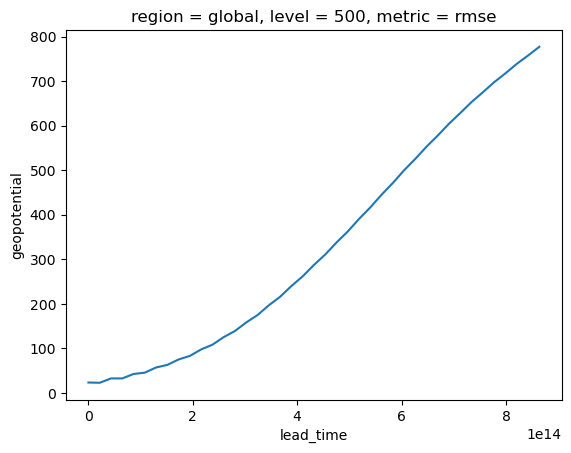
Note that to compute the RMSE, we follow ECMWF’s convention by taking the square root after the time mean. To do this in WB2, first compute the MSE and then take the square root of the saved MSE results.
results = xr.concat(
    [
    results,
    results.sel(metric=['mse']).assign_coords(metric=['rmse']) ** 0.5
    ],
    dim='metric'
)
results['geopotential'].sel(metric='rmse', level=500, region='global').plot();
Next steps
This quickstart guide shows the basic functionality of the WeatherBench evaluation code but there is more to explore.
For running evaluation from the command line, see this guide. For a complete overview of the entire evaluation workflow, check out the “submission” guide.